
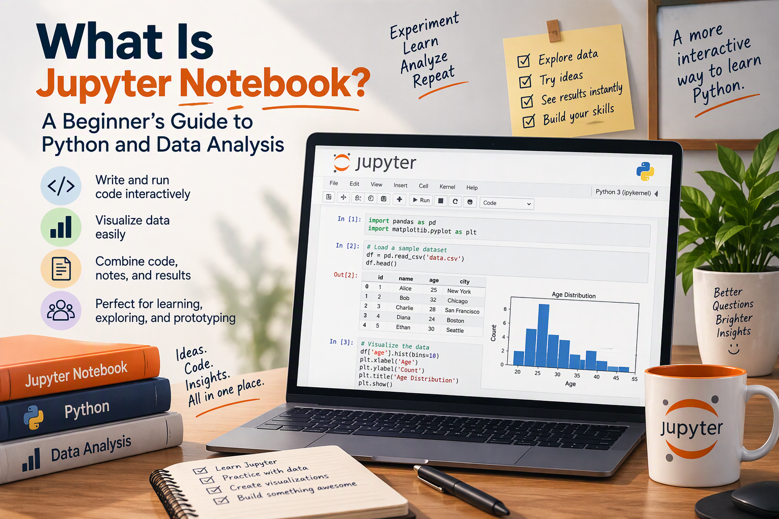
If you’ve followed a Python data analysis tutorial, taken an online data course, or looked at a data scientist’s project on GitHub, you’ve almost certainly seen a Jupyter Notebook. It’s the tool where code, results, charts, and explanations all live together on one page, and it’s the most popular way to explore data with Python.
In this guide, you’ll learn what Jupyter Notebook is, how to install it, how its cells work, and how to use it for a real (small) data analysis with Pandas. You’ll also learn the keyboard shortcuts and “magic commands” that make it faster, plus the habits that keep your notebooks clean and reliable.
What Is Jupyter Notebook?
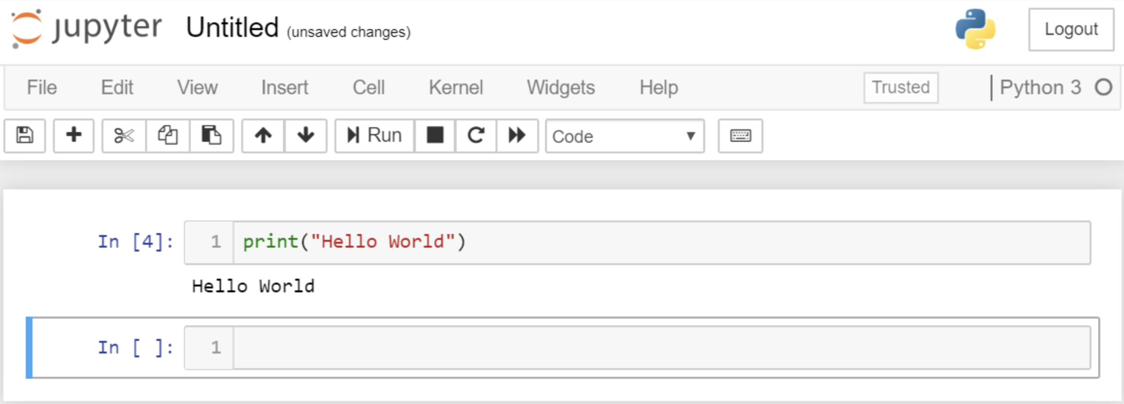
Jupyter Notebook is a free, open-source application that lets you write and run code in small pieces, called cells, right in your web browser. Each cell’s result, whether a number, a table, or a chart, appears directly below it. Between the code cells, you can write formatted text, headings, and lists to explain what you’re doing.
The result is a document that tells a story: here’s the question, here’s the code, here’s what it showed, and here’s what it means. That’s why it’s so popular for data analysis, teaching, and sharing research.
A few key ideas:
- Notebook file: notebooks are saved as
.ipynbfiles (short for Interactive Python Notebook). The file stores your code, your text, and your outputs, so someone can read your results without running anything. - Cells: the building blocks of a notebook. Code cells contain code; Markdown cells contain formatted text.
- Kernel: the “engine” running your code in the background. For Python, it’s an IPython process. The kernel remembers everything you’ve run until you restart it, which is what lets one cell use a variable created in another.
- The name: Jupyter comes from three of the first languages it supported: Julia, Python, and R. Today it supports dozens of languages, but Python is by far the most common.
Why Data Analysts Use Jupyter
- Instant feedback. Run one step, look at the result, adjust, and run it again, without rerunning the whole script. That’s exactly how data exploration works.
- Results right next to the code. Tables and charts appear below the code that made them, so you never lose track of which output came from where.
- Documentation built in. Markdown cells let you explain your reasoning, so the notebook doubles as a report.
- Easy to share. GitHub displays
.ipynbfiles with their outputs, and you can export a notebook to HTML or PDF. - Great for learning. You can break a problem into small steps and see what each line does.
(New to data analysis as a career? See What Is a Data Analyst?.)
Jupyter Notebook vs. JupyterLab vs. Other Options
You’ll see several names. They all use the same .ipynb file format:
| Tool | What it is | Best for |
|---|---|---|
| Jupyter Notebook | The classic, simple interface: one notebook per browser tab | Beginners and focused work |
| JupyterLab | The newer, full-featured interface, with a file browser, tabs, a terminal, and side-by-side panels | Day-to-day work on larger projects |
| Google Colab | A free, hosted notebook in your browser; nothing to install | Trying Jupyter instantly, or using free GPUs |
| VS Code | A code editor with built-in notebook support | People who already code in VS Code |
If you’re not sure, start with Jupyter Notebook or Google Colab. Everything in this guide works in all of them.
How to Install Jupyter Notebook
You’ll need Python 3 installed. The best practice is to install Jupyter inside a virtual environment, so each project keeps its own packages. (See Python Virtual Environments: Setup Guide & Best Practices.)
Option 1: pip
On macOS or Linux:
python3 -m venv .venv
source .venv/bin/activate
pip install notebook pandas matplotlib
jupyter notebook
On Windows, activate the environment with .venv\Scripts\activate instead, and use python instead of python3.
The last command starts a local Jupyter server and opens the dashboard in your browser: a file browser showing the folder you started it from. Click New → Python 3 (ipykernel) to create a notebook. Leave the terminal window open while you work; closing it stops Jupyter.
For JupyterLab, install jupyterlab and run jupyter lab instead.
Option 2: uv
If you use uv, you can launch JupyterLab without installing it into your project at all:
uv run --with jupyter jupyter lab
Option 3: Anaconda
The Anaconda distribution installs Python, Jupyter, Pandas, and hundreds of data science packages in one download. It’s convenient but large; the pip and uv options above give you more control.
Understanding Cells
Every notebook is a list of cells. You’ll use two kinds:
- Code cells run code and show the output below. To the left, you’ll see
[ ]before the cell runs,[*]while it’s running, and a number like[3]after it runs. The number tells you the order in which cells were run. - Markdown cells hold formatted text: headings (
#), bold (**text**), lists, links, and even tables. Run a Markdown cell to render it.
To run a cell, click inside it and press Shift + Enter. Jupyter runs it and moves to the next cell.
Your First Notebook
Create a new notebook and type this into the first cell, then press Shift + Enter:
2 + 2
4
Jupyter automatically displays the value of the last line of a cell, so you don’t need print() for a quick check. You can still use print() when you want to show something in the middle of a cell, or more than one thing:
name = "Jupyter"
print(f"Hello, {name}!")
Hello, Jupyter!
Now, in a new cell:
name.upper()
'JUPYTER'
This works because the kernel remembers the name variable from the previous cell. Everything you run stays in memory until you restart the kernel. That’s what makes notebooks so convenient, and, as you’ll see later, it’s also their biggest trap. (If you’re new to Python itself, start with Python Basics: What Every Beginner Should Know.)
Analyzing Data in a Notebook
Here’s where Jupyter shines. This example uses the online store dataset from SQL and Data Science Interview Questions; download the CSV files from that post and put them in the same folder as your notebook.
Load the data and look at it:
import pandas as pd

orders = pd.read_csv("orders.csv")
orders.head()
   order_id  customer_id  order_date     status
0       101            1  2025-08-02  completed
1       102            2  2025-08-05  completed
2       103            1  2025-08-19  completed
3       104            3  2025-08-21  cancelled
4       105            4  2025-09-01  completed
In Jupyter, a DataFrame displays as a nicely formatted HTML table; the text above shows the same content.
Check its size and count orders by status, each in its own cell:
orders.shape
(60, 4)
orders["status"].value_counts()
status
completed    48
cancelled     6
pending       6
Name: count, dtype: int64
Combine tables and calculate revenue by category. Notice how this cell reuses orders and pd from earlier cells:
items = pd.read_csv("order_items.csv")
products = pd.read_csv("products.csv")

sales = items.merge(products, on="product_id").merge(orders, on="order_id")
completed = sales[sales["status"] == "completed"].copy()
completed["revenue"] = completed["quantity"] * completed["price"]

by_category = completed.groupby("category")["revenue"].sum().sort_values(ascending=False)
by_category
category
Home Office    4825.0
Electronics    4200.0
Stationery      469.5
Accessories     435.0
Name: revenue, dtype: float64
Plot it. Charts appear right below the cell:
by_category.sort_values().plot(kind="barh", title="Revenue by Category (Completed Orders)");
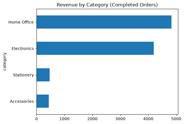
The semicolon at the end hides a line of text (<Axes: ...>) that Jupyter would otherwise display along with the chart.
In a few small cells, you went from raw CSV files to a finding: Home Office and Electronics bring in more than 90% of the revenue. If you added a Markdown cell explaining that, your notebook would already be a small report. (To go further, see Data Cleaning with Python Pandas and Python Data Visualization.)
Keyboard Shortcuts
Jupyter has two modes, and shortcuts depend on which one you’re in:
- Edit mode (press Enter or click inside a cell): you’re typing inside the cell.
- Command mode (press Esc): you’re working with cells as blocks: adding, deleting, and moving them.
| Shortcut | Mode | What it does |
|---|---|---|
| Shift + Enter | Both | Run the cell and move to the next one |
| Ctrl + Enter | Both | Run the cell and stay on it |
| Alt + Enter | Both | Run the cell and insert a new one below |
| A / B | Command | Insert a cell above / below |
| D, D (press twice) | Command | Delete the cell |
| Z | Command | Undo a cell deletion |
| M / Y | Command | Change the cell to Markdown / code |
| C / X / V | Command | Copy / cut / paste cells |
| Tab | Edit | Autocomplete names |
| Shift + Tab | Edit | Show the documentation for a function |
On a Mac, use Cmd where a shortcut uses Ctrl for copying and saving, but Ctrl + Enter stays the same for running a cell.
Magic Commands
Magic commands are special Jupyter commands that start with % (for one line) or %% (for the whole cell). They aren’t Python, but they’re very handy:
| Magic | What it does |
|---|---|
%pip install pandas | Installs a package into the environment the notebook is running in |
%timeit expression | Times a short piece of code by running it many times |
%%time | Times the whole cell, run once (put it on the first line) |
%who | Lists the variables currently in memory |
%run script.py | Runs a Python file and loads its variables into the notebook |
%%writefile name.py | Saves the contents of the cell to a file |
For example:
%timeit sum(range(1000))
19.7 μs ± 422 ns per loop (mean ± std. dev. of 7 runs, 10,000 loops each)
Your numbers will be different; they depend on your computer.
A line starting with ! runs a terminal command instead, like !ls (or !dir on Windows). For installing packages, though, prefer %pip over !pip: !pip can install into a different Python than the one your notebook uses, which leads to confusing “module not found” errors.
The Biggest Trap: Hidden State
Because the kernel remembers everything, a notebook can reach a state that no longer matches the code you see. For example:
- You run a cell that creates
total = 100. - You delete that cell.
- Another cell that uses
totalstill works, becausetotalis still in memory.
The next time you (or anyone else) open the notebook and run it from the top, it fails. The same thing happens when you run cells out of order, or edit a cell and forget to rerun the ones after it. Execution numbers like [7], [3], [12] out of order are a warning sign.
The fix: before you trust or share a notebook, use Kernel → Restart Kernel and Run All Cells. If it runs cleanly from top to bottom, your results are reproducible.
Best Practices for Clean Notebooks
- Restart and run all before sharing or trusting your results.
- Put imports and settings at the top, in the first cell.
- Use Markdown headings to split the notebook into sections: question, data, analysis, conclusion.
- Give each cell one job. Short cells are easier to read, rerun, and debug.
- Never put passwords or API keys in a notebook. Outputs and code are saved in the file, and it’s easy to push them to GitHub by accident. Load secrets from a
.envfile instead. (See The Importance of the .env File in Python Projects.) - Clear large outputs before committing to Git. Use Edit → Clear Outputs of All Cells to keep files small and diffs readable. (See Mastering Git: Basic Commands.)
- Move reusable code into
.pyfiles. When a function grows or you need it in several notebooks, put it in a module and import it.
Sharing and Exporting Notebooks
- GitHub renders
.ipynbfiles with their outputs, so others can read your analysis right in the browser. - Google Colab can open notebooks straight from GitHub or Google Drive, so others can run them without installing anything.
- Export to HTML from File → Save and Export Notebook As → HTML, or from the terminal:
jupyter nbconvert --to html my_analysis.ipynb
This creates my_analysis.html, which anyone can open in a browser without Python. Export to PDF is also available, but it requires extra software (such as LaTeX).
When Not to Use a Notebook
Notebooks are ideal for exploring, learning, and explaining. They’re not the best fit for:
- Production code that runs on a schedule, like a nightly data pipeline. Use regular
.pyscripts. - Large applications, like a web app. (See Python Flask: A Complete Guide.)
- Code that needs automated tests, which are much easier to write for
.pymodules.
A common workflow is to explore in a notebook, then move the finished logic into scripts.
Conclusion
Jupyter Notebook combines code, results, charts, and explanations in one document, which makes it the go-to tool for exploring data with Python. You learned how to install it, how code and Markdown cells work, how the kernel keeps variables between cells, how to analyze a real dataset with Pandas, and how to work faster with shortcuts and magic commands.
Most importantly, remember the one habit that separates reliable notebooks from confusing ones: restart the kernel and run everything from the top before you trust your results. Now open a new notebook, load a dataset you’re curious about, and start asking it questions.